
Singapore Retail Sales Forecasting Project (Python, ML, Tableau)
Date Posted: 2025-06-03
Category: Data Projects
Project Objectives
This project aims to predict monthly retail sales (in million SGD) in Singapore using machine learning. The goal is to provide accurate and interpretable forecasts that could help businesses and policymakers anticipate market demand, allocate inventory more effectively, and make data-driven decisions.
Specific objectives include:
- Feature Engineering: Exploring adding various time-step features and exogenous variables for machine learning model
- Prediction & Accuracy: Evaluate the efficacy of using machine learning in forecasting retail sales in SG, and create predictions along with visualizations for simple & effective presentation
- Visualization & Communication: Present insights and forecasts through dashboards using Tableau
The full code can be found below:
Dataset
In this analysis, I used the SingStat Table Builder from Department of Statistics, Singapore (DOS) to retrieve 29 years of monthly retail sales data for Singapore from 1997 to 2025.
Preprocessing the Dataset
Outlier Analysis
COVID-19 caused heavy drop in retail sales. We created an indicator feature [‘is_covid’] for the machine learning algorithm to identify the COVID-19 period as outliers, ensuring that the model can account for these outliers.
###Adding COVID-19 indicator feature
df['is_covid'] = df.index.to_series().between('2020-04', '2020-06').astype(int)
Feature Engineering
Creating time-step features: ‘month’, ‘quarter’ and ‘year’.
#Time Step Features
def create_features(df):
    """
    Creates time-step features (month, quarter, year) from the DataFrame's index.

    Args:
        df (pd.DataFrame): The input DataFrame with a DatetimeIndex.

    Returns:
        pd.DataFrame: The DataFrame with added time-step features.
    """
    df_copy = df.copy()

    # df_copy['hour'] = df_copy.index.hour # Uncomment if needed
    # df_copy['dayofweek'] = df_copy.index.dayofweek # Uncomment if needed
    df_copy['month'] = df_copy.index.month
    df_copy['quarter'] = df_copy.index.quarter
    df_copy['year'] = df_copy.index.year
    # df_copy['dayofyear'] = df_copy.index.dayofyear # Uncomment if needed

    return df_copy

df = create_features(df)
With time-step features, we can do some visualisations to investigate signs of trends and/or seasonality
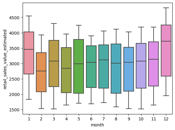
We also created lag features: ‘sales_lag_1’ and ‘sales_lag_2’
#Lag Features
df['sales_lag_1'] = df['retail_sales_value_estimated'].shift(1)
df['sales_lag_2'] = df['retail_sales_value_estimated'].shift(2)
We assessed that lag features were unsuitable and worsened prediction results instead.
Model Building
Time Series Cross Validation
We used the TimeSeriesSplit module to conduct time series cross validation by creating n folds to assess the efficacy of using time series forecasting for retail sales values. This method helps to prevent lookahead bias by repeatedly evaluating a different set of 12 months towards the end of the dataset.
It should be worth considering that our dataset is quite small, so it will be expected to see natural improvements as 12 datarows worth of data are added after each fold.
We used parameters n_split = 3 & test_size = 12.
tss = TimeSeriesSplit(n_splits = 3, test_size = 12
                      , gap = 0)
XGBoost Regression
We used the XGB Reg module to build our model.
tss = TimeSeriesSplit(n_splits = 3, test_size = 12
                      , gap = 0)

fold = 0
preds = []
scores = []
for train_idx, val_idx in tss.split(df):
    train = df.iloc[train_idx]
    test = df.iloc[val_idx]

    train = create_features(train)
    test = create_features(test)

    FEATURES = ['quarter', 'month', 'year','is_covid']
    TARGET = 'retail_sales_value_estimated'

    X_train = train[FEATURES]
    y_train = train[TARGET]

    X_test = test[FEATURES]
    y_test = test[TARGET]

    reg = xgb.XGBRegressor(base_score=0.5, booster='gbtree',
                           n_estimators=1000,
                           early_stopping_rounds=50,
                           objective='reg:linear',
                           max_depth=3,
                           learning_rate=0.01)
    reg.fit(X_train, y_train,
            eval_set=[(X_train, y_train), (X_test, y_test)],
            verbose=100)

    y_pred = reg.predict(X_test)
    preds.append(y_pred)
    score = np.sqrt(mean_squared_error(y_test, y_pred))
    scores.append(score)
Model initial evaluation
The RMSE results of the folds were: Score across folds: 132.5939 Fold scores:[147.9255505042701, 138.56629972923642, 111.28990440456352]
The image below shows the model’s prediction against the actual data for dates past 2024.
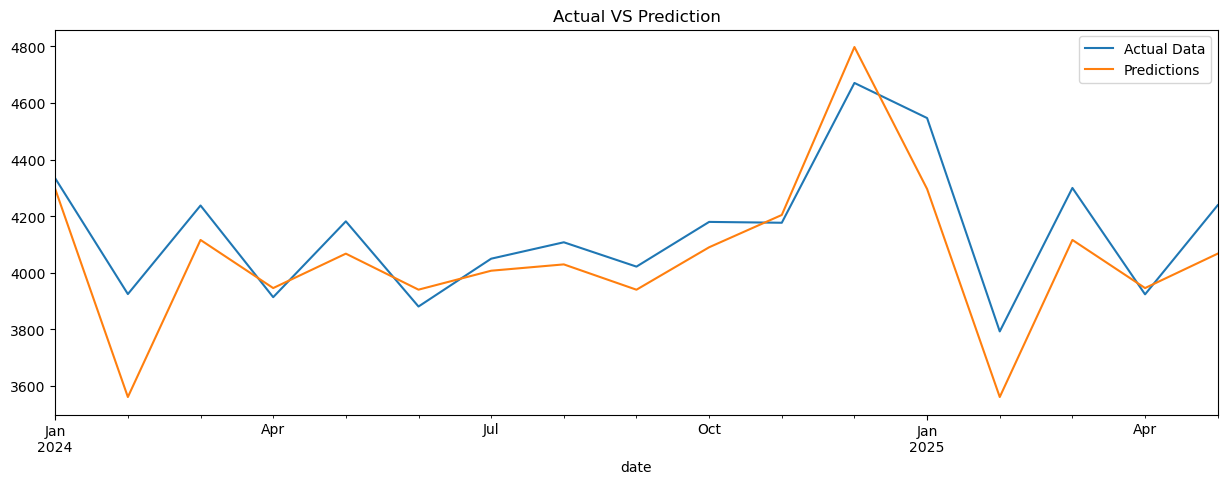
As we can see, the model has generally done well to capture the monthly seasonality of retail sales in SG, capturing the shape without too much of an error.
Prediction & Visualisation
Final Model & Forecasting
#Final Model Building

FEATURES = ['quarter', 'month', 'year', 'is_covid']
TARGET = 'retail_sales_value_estimated'

X_full = df[FEATURES]
y_full = df[TARGET]
reg = xgb.XGBRegressor(
base_score=0.5,
booster='gbtree',
n_estimators=1000,
early_stopping_rounds=50,
objective='reg:squarederror', # use this instead of 'reg:linear' (deprecated)
max_depth=3,
learning_rate=0.1
)
reg.fit(X_full, y_full, eval_set=[(X_full, y_full)], verbose=100)Tableau Visualisation
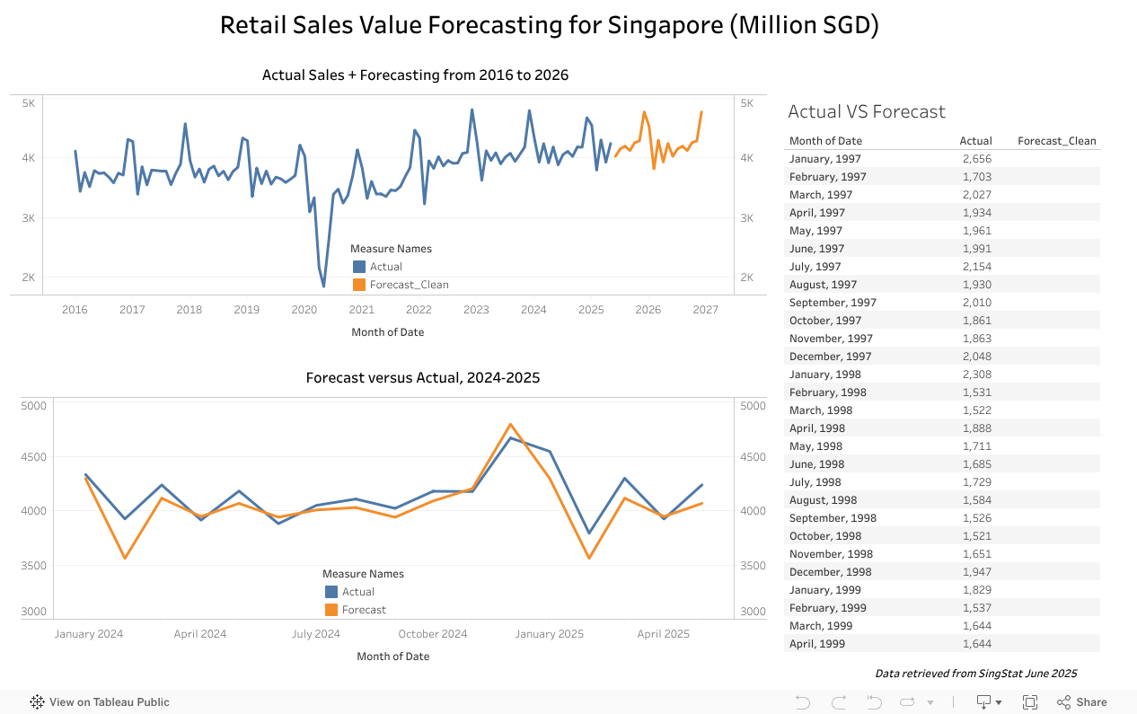
We then visualised the actual & forecasted data in Tableau.
Conclusion
Using machine learning models to predict retail sales forecasting showed some promise as seen in the results of the time series cross validation. It is worth acknowledging that this dataset is lacking in volume, both in terms of depth and breadth. There could be more data points, i.e. using weekly or even daily sales for analysis, and there could be more exogenous variables such as promotions, holidays, etc.