Breast Cancer Classification with Logistic Regression, CART, and Random Forest (R)

Date Posted: 2025-03-03

Category: Data Projects

In this analysis, I used the Wisconsin Breast Cancer Dataset to build and evaluate models for classifying tumors as benign or malignant. This project demonstrates a complete machine learning pipeline in R, including:

• Data cleaning and feature selection
• Correlation analysis
• Model training and tuning
• Handling class imbalance via sampling
• Comparison of model performance (Logistic Regression, CART, Random Forest)

Project Objectives

The primary objective of this project was to investigate the efficacy of using ML models to assist in breast cancer diagnosis. Besides that, I also look into:

1. Feature Selection through variable importance
2. Methods of handling class sampling
3. Hyper-parameter tuning in RandomForest

The full code can be found below:

View Notebook

Dataset

The dataset comes from the UCI Machine Learning Repository and contains numerical features computed from digitized images of breast masses. Key features include radius, texture, perimeter, area, and more — measured via mean, standard error, and worst-case metrics.

Preprocessing the Dataset

Removing Multicollinear Variables

To avoid multicollinearity, I used findCorrelation() from the caret package to identify and remove highly correlated variables (threshold > 0.8).

corr1 <- cor(data.dt)
corrplot(corr1,type = 'lower', method = 'color', ...)

to_drop <- c("concavity_mean", "compactness_mean", ...)
initial_data <- select(data.dt, -to_drop)

initial_data$diagnosis <- factor(initial_data$diagnosis)

The target variable was also factorised to prepare for classification tasks.

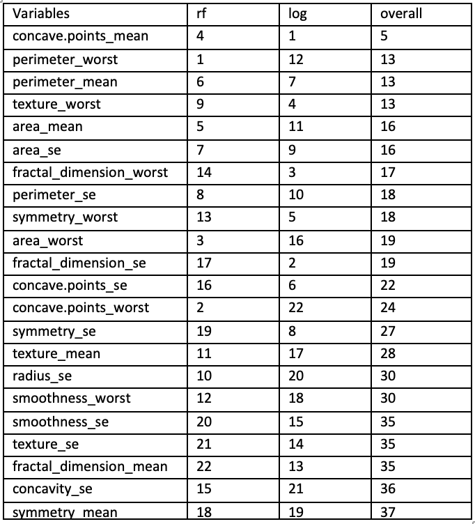
Feature Importance

To identify the most influential features, a baseline logistic regression and a random forest model was trained initially.

logmodel1 <- glm(diagnosis ~ ., data = initial_data, family = binomial())
vim1 <- varImp(logmodel1)

rf_model1 <- randomForest(diagnosis ~ ., data = initial_data)
vim2 <- varImp(rf_model1)

The feature importance values were exported and reviewed in Excel to guide further feature reduction.

Model Building

Logistic Regression

logmodel1 <- glm(diagnosis~.,data=trainset,family=binomial())
summary(logmodel1)

#Remove insignificant variables
logmodel2 <- glm(diagnosis ~ perimeter_mean + concave.points_mean+ texture_worst + symmetry_worst,data=trainset,family=binomial())
summary(logmodel2)

#Evaluate model with confusion matrix
logmodel2.test<-predict(logmodel2,newdata=testset,type='response')

#threshold = 0.9
logmodel2.predict.test<-ifelse(logmodel2.test>0.9,"1","0")

Decision Tree (CART)

We use CART decision tree (pruned using cross-validated CP)

#Cart
set.seed(100)
Cart1  <- rpart(diagnosis ~.,data=trainset, method='class', control = rpart.control(minsplit = 2, cp=0.0))

print(Cart1)
#Viewing prune sequences, prune triggers, and 10-fold CV errors
printcp(Cart1)

#Identifying optimal CP with plotted CP
plotcp(Cart1)
cp1 = sqrt(0.0135135*0.0090090)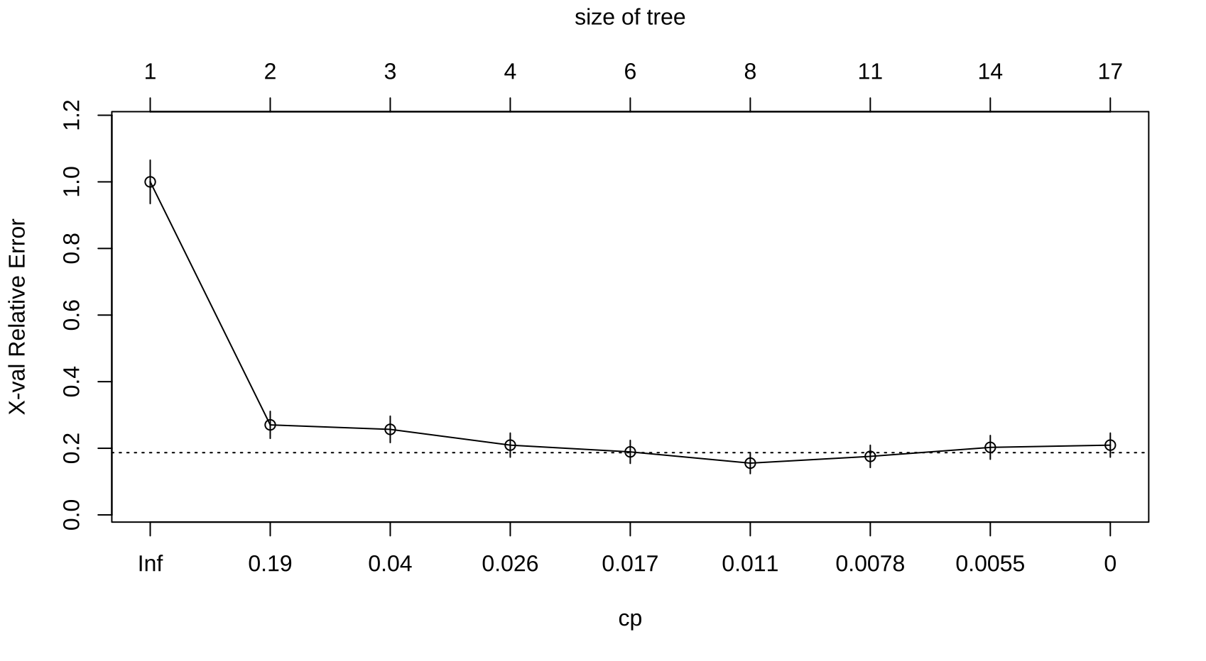

#Pruning tree at cp = 0.01103373
cp1 = sqrt(0.006*0.008)
cp1
Cart2<-prune(Cart1,cp=cp1)
printcp(Cart2)

rpart.plot(Cart2, nn= T, main = "Pruned Tree with cp = 0.006928203")
Cart2$variable.importance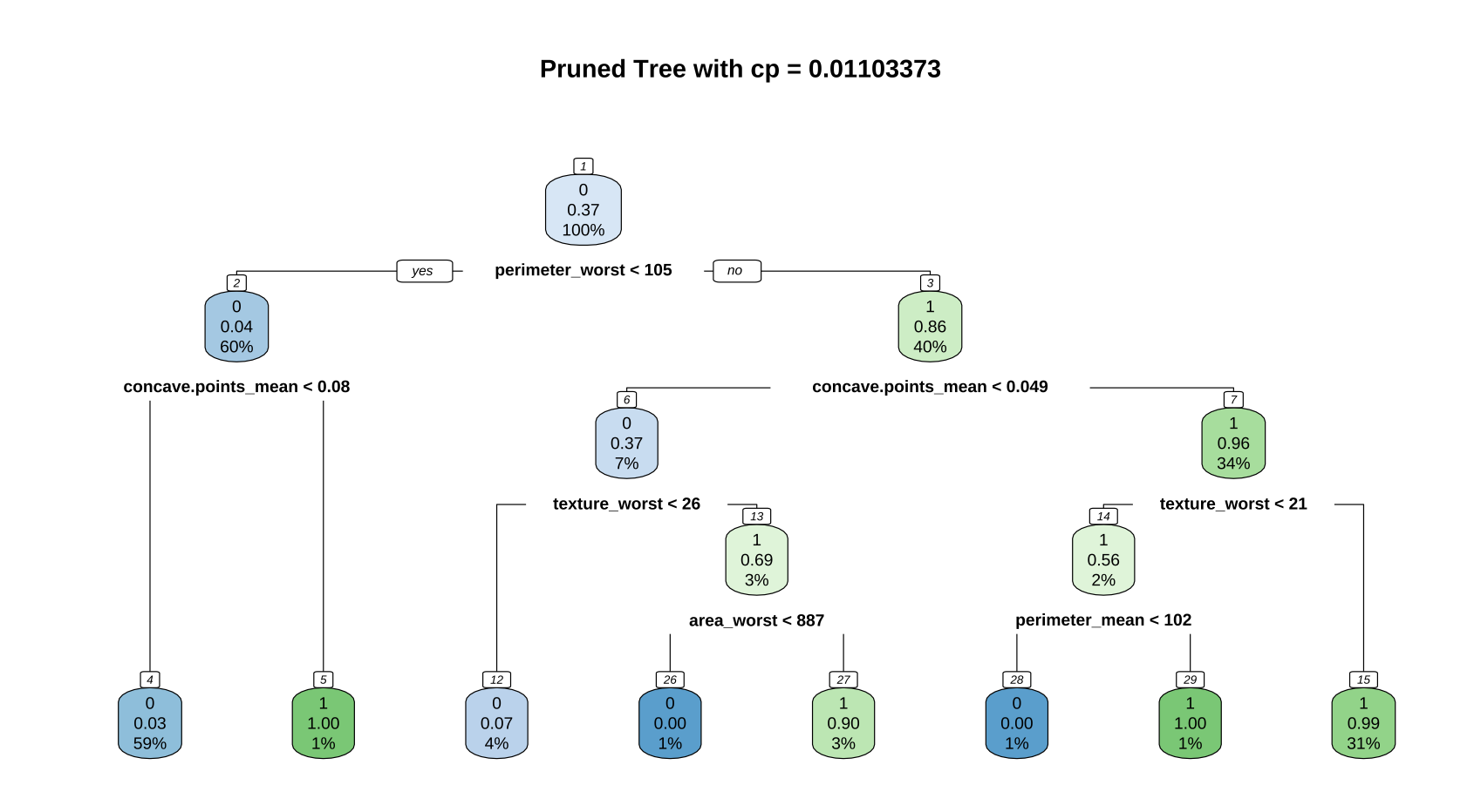

RandomForest Model

Random Forest Tuning

I implemented a custom loop to test various mtry and ntree combinations and recorded their test set accuracy.

rf_parameter_test <- function(mtry, ntree) {
randomForest(diagnosis ~ ., data = trainset, mtry = mtry, ntree = ntree)
}

for (mtry in 1:ncol(trainset) - 1) {
for (ntree in c(25, 100, 500)) {
model <- rf_parameter_test(mtry, ntree)
accuracy <- mean(predict(model, testset) == testset$diagnosis)
}
}

You can find the parameters and their results below:

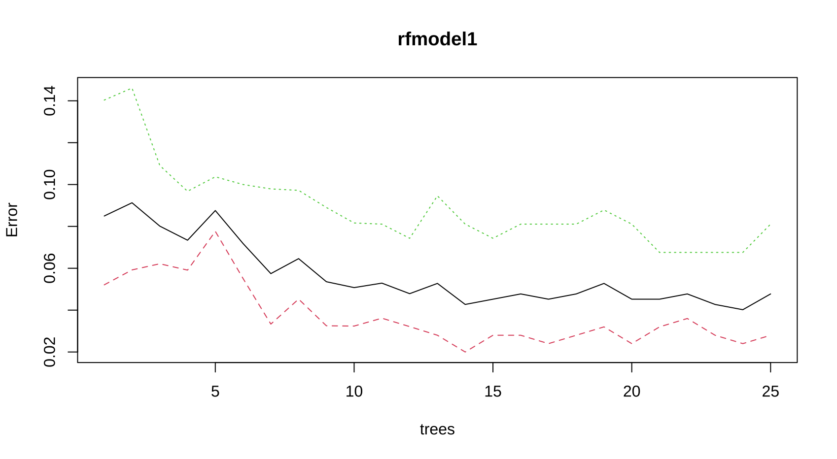
Proceeded with RSF = 6 and B = 25, as they performed well across both seeds. We use the tuned RandomForest Model, with RSF = 6 and B = 25.

set.seed(100)
rfmodel1 <-randomForest(trainset$diagnosis~ ., data = trainset, importance = T, ntree = 25,mtry =6) 
rfmodel1 
var.impt <- importance(rfmodel1)

varImpPlot(rfmodel1, type = 1)

plot(rfmodel1)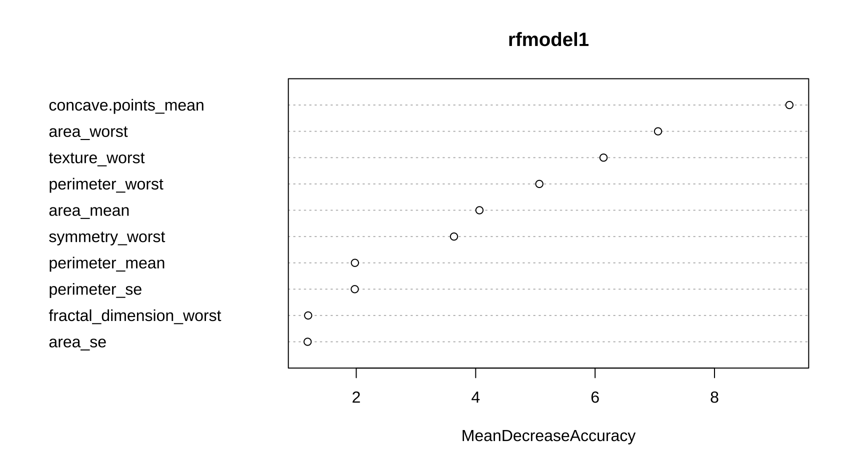

Balancing Data

Data is imbalanced, with relatively more benign diagnosis. Data imbalances can lead to issues such as overfitting, or the end-model having inaccuracy in identifying cases (benign, in this context) with less observations.

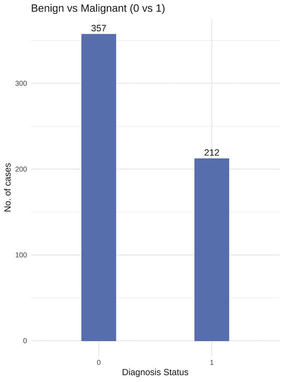
We will investigate the effects of upsampling/downsampling with the original dataset as a control.

The downsampling/upsampling methods can be found below.

#Balanced dataset, downsampled
trainset <- downSample(trainset,trainset$diagnosis)
View(trainset)
table(trainset$diagnosis)

#Balanced dataset, upsampled
trainset <- upSample(trainset_original,trainset_original$diagnosis)
View(trainset)
table(trainset$diagnosis)

After generating the various balanced datasets, we repeated the above process of building the 3 models and compared the results:

Overall Evaluation

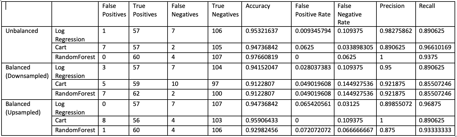
We can see that models that used data that was upsampled generally did better than downsampled data. This is likely due to the dataset being very small. Even a few sets of data being downsampled was relatively more significant information loss for the models.

In the context of breast cancer diagnosis, false negatives are the most dangerous outcomes as they mean a person with cancer has gone undetected; logmodel generally had the best performance when it came to

RandomForest generally had the best performance in terms of accuracy and the various metrics.

Conclusion

This project demonstrated the importance of:

• Careful feature selection to reduce multicollinearity
• Tuning hyperparameters for tree-based models
• Handling class imbalance in medical data
• Comparing multiple models for both interpretability and accuracy

In real-world applications like cancer diagnosis, model choice and threshold tuning have life-and-death implications. Balancing recall and precision is vital.

This project shows that there is some efficacy in using ML models to diagnose breast cancer. It is also worth noting that certain features carried much of the predictive power - for example, concave.points_mean. However, the dataset is small, and it is recommended that future projects use a larger dataset for a more accurate evaluation of ML models for breast cancer diagnosis.