
Store Sales Forecasting (Python)
Date Posted: 2025-04-22
Category: Data Projects
In this page I practice forecasting, feature engineering, and using various regression and machine learning models.
Store Sales Forecasting
This project uses the Store Sales Dataset from Kaggle. The goal of this project is to optimize inventory for the store Favorita in Ecuador. The desired outcomes are to:
- Reduce Waste (By reducing wasted inventory)
- Improving customer satisfaction by ensuring inventory is always adequate
- Reduce inventory holding costs
This starts with having accurate forecasts to optimize inventory to reduce waste and holding costs.
The full .ipynb file(s) can be found in the link below.
Exploratory Data Analysis
First, we take a look at the store sales data.
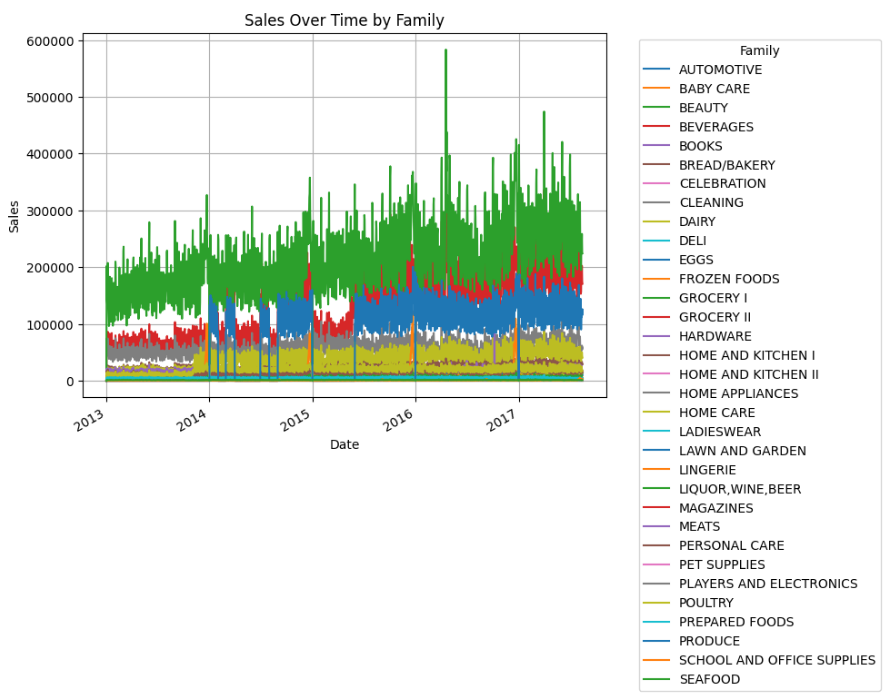
The dataset is quite large, and each family (category) varies in volume purchased. We’ll take a closer look by plotting after aggregating using family instead.
From the image above, we can see that there are clear inconsistencies / missing data in the dataset, especially so pre June 2015. Regression and Machine Learning Models likely won’t be able to capture useful information if we include those dates, and thus we will focus on data post June 2015.
Methodology
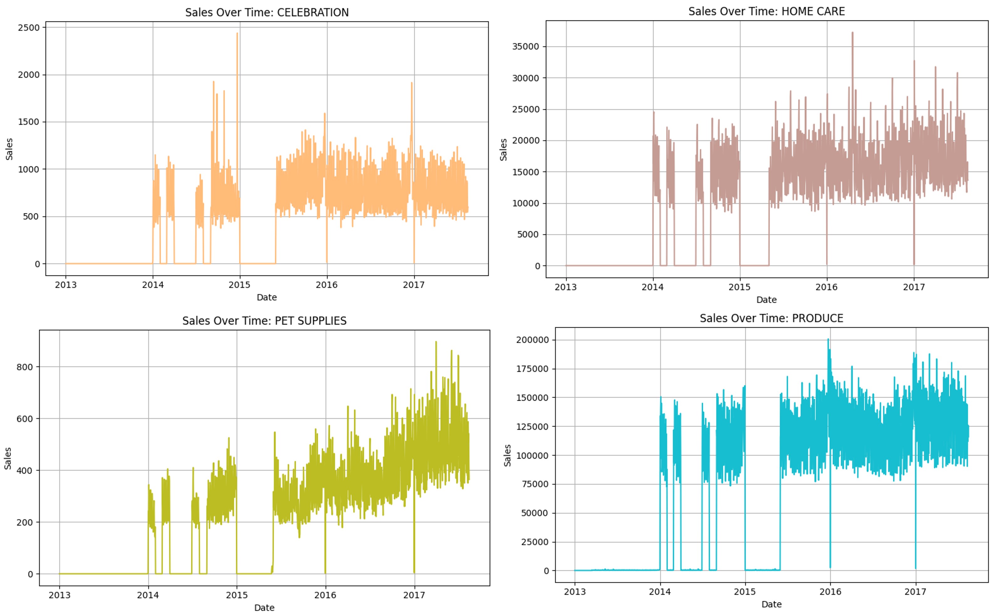
As a proof of concept, we investigate the credibility of our methods by building some forecasts from datasets with a good amount of sales. We will work with categories ‘Produce’ and ‘Poultry’.
We will use the SARIMAX model for time series forecasting. We expect strong weekly seasonality since Favorita sells daily goods.
Model Building
As we are using an ARIMA model, we check for stationarity with Augmented Dickey-Fuller (ADF) test.
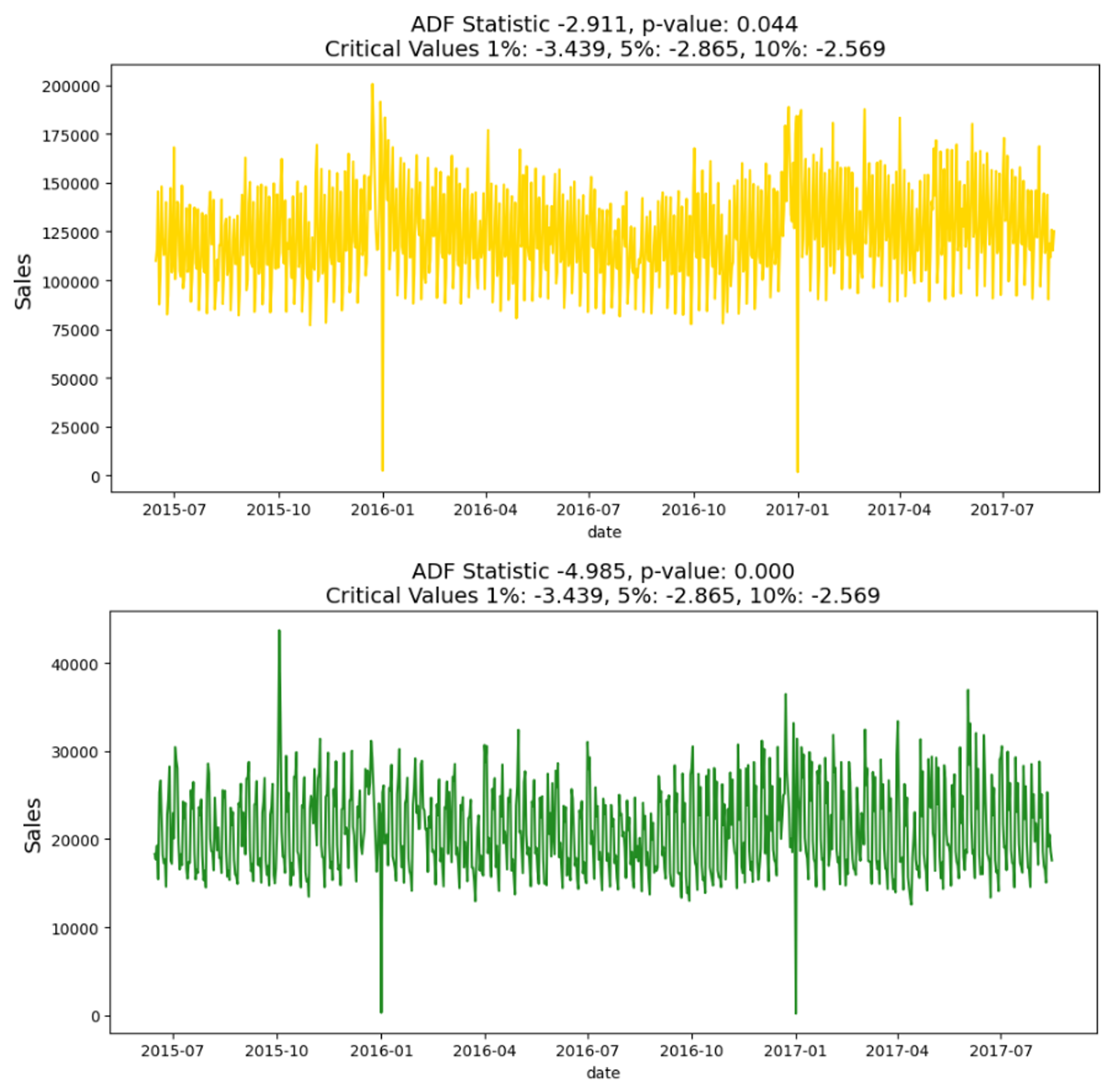
Both datasets were within the acceptable range to be stationary.
We then plotted the auto-correlation (ACF) and partial auto-correlation (PACF) plots to investigate the AR & MA.
Initial inspection of the ACF and PACF plots revealed that although data was stationary according to the ADF test, it was not seasonally stationary. With spikes at 7, 14, 21… , we can clearly see strong weekly seasonality as expected. The following are the ACF and PACF plots after differencing for the weekly seasonality.
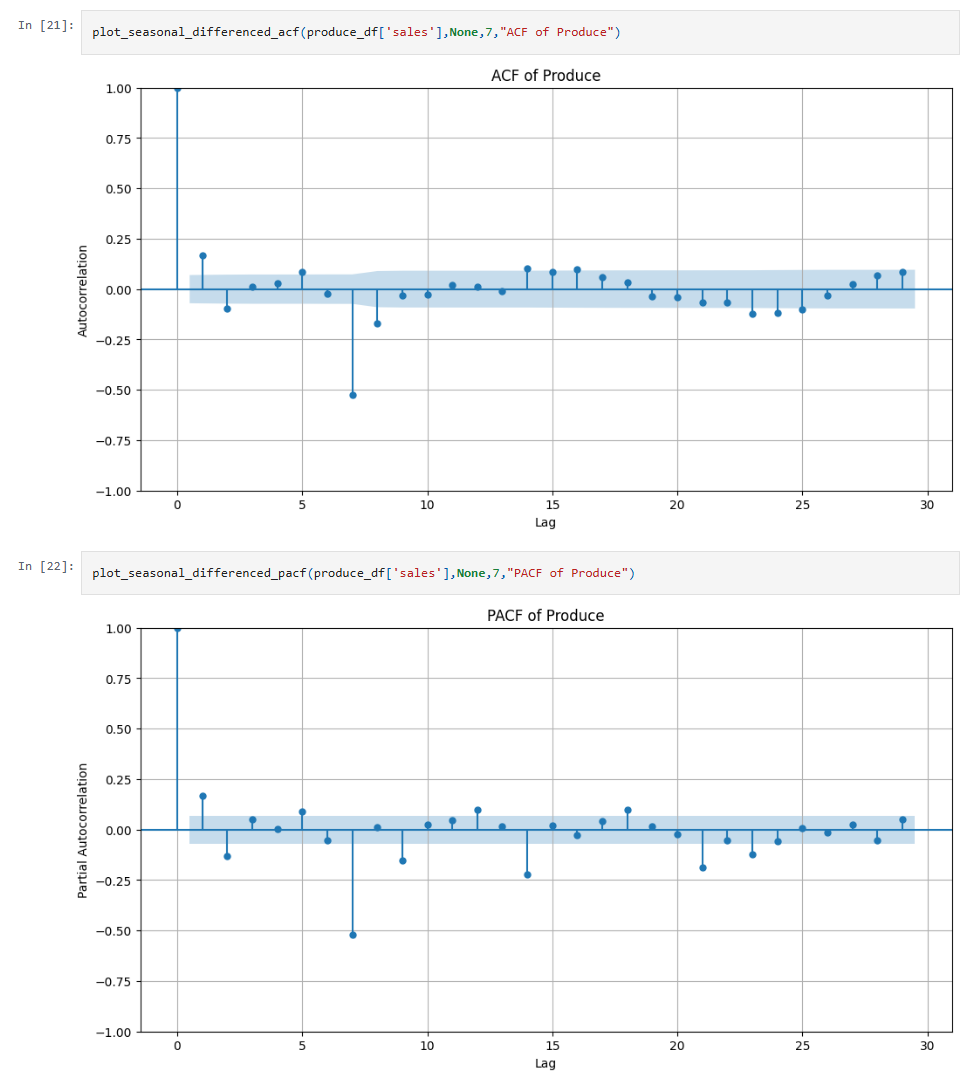
We use these plots to identify candidates orders for the p & q components of the ARIMA model. For example, since information drops off after lags 1 & 2, we do a grid search with range 0-2 for both p & q.
Here are some snippets from my grid search:
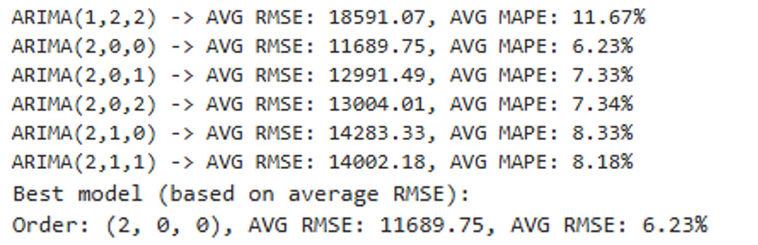
For sales data under category ‘produce’, we arrived at p,d,q values of 2,0,0 for the ARIMA model, along with 1,0,1,7 for the seasonal component.
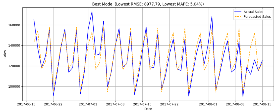
Followed by an example forecast from initial train-test-split using test data as last 2 months and earlier dates as training data.
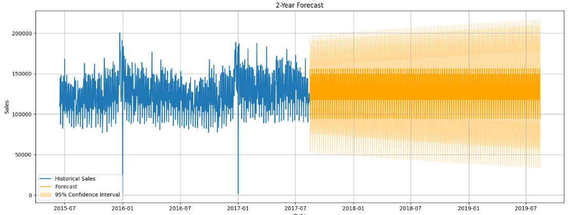
Finally, we have an example future 2-year forecast using, all of the data, inclusive of the 2 months we initially used as test data.
Evaluation
Since we lack actual future data, we’ll evaluate using RSME and MAPE.
As previously shown, training against data from 2015-06-15 to 2017-06-14 and using 2017-06-15 to 2017-08-15 yielded an average RMSE of 11689.75 with an average MAPE of 6.23%, suggesting that the forecasts are highly accurate.
Residuals
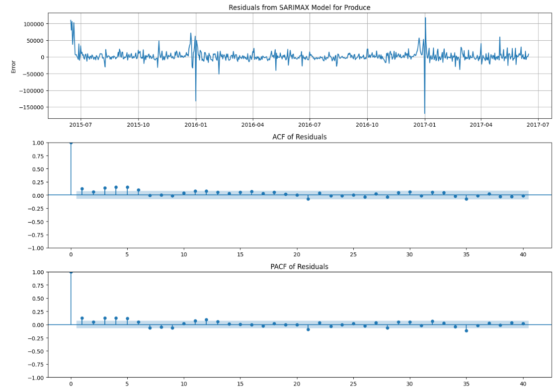
Lastly, we have the residual plots. Ideally, they should be completely random.
We can see that there is information that the model has not captured since both plots are not fully within the confidence band. This could be due to lack of exogeneous variables for the model. If favorita wishes to work with us and provides us with even more information, we can build an even more accurate model.
Implementation
Based on these PoC results, we believe that implementing forecasting model can lead to savings from reduced inventory holding costs and reducing wasted inventory. Customer Satisfaction will also improve due to reduced instances of stockouts.
Recommendations
We recommend a pilot program focused on a few categories first. By focusing on a few categories with an ample amount of sales data and including other variables such as promotion data, we can further refine models for forecasting for all categories.
If performance is within acceptable ranges for 2 months, forecasts can potentially be used in determining inventory to order and forecasting can be implemented for more categories.
To scale up, we can prepare automated date infrastructure that will automatically retrieve exogeneous variables from sales data to be fed into the pipeline to create forecasts in real-time.